Frequency table for categorical and continuous data and returns the
frequency, cumulative frequency, frequency percent and cumulative frequency
percent. plot.ds_freq_table() creates bar plot for the categorical
data and histogram for continuous data.
Usage
ds_freq_table(data, col, bins = 5)

# S3 method for class 'ds_freq_table'
plot(x, print_plot = TRUE, ...)Examples
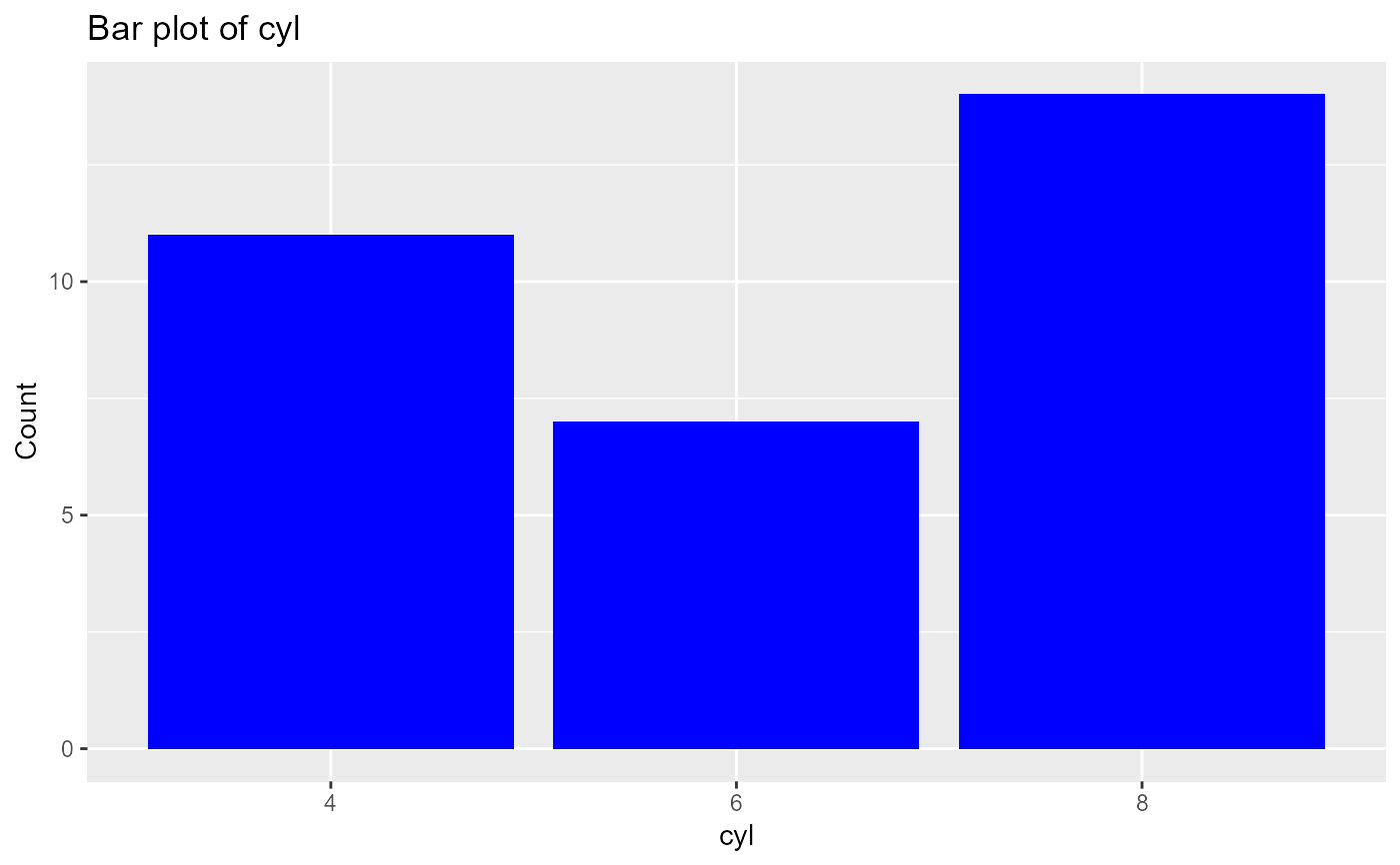
# categorical data
ds_freq_table(mtcarz, cyl)
#> Variable: cyl
#> -----------------------------------------------------------------------
#> Levels Frequency Cum Frequency Percent Cum Percent
#> -----------------------------------------------------------------------
#> 4 11 11 34.38 34.38
#> -----------------------------------------------------------------------
#> 6 7 18 21.88 56.25
#> -----------------------------------------------------------------------
#> 8 14 32 43.75 100
#> -----------------------------------------------------------------------
#> Total 32 - 100.00 -
#> -----------------------------------------------------------------------
#>
# barplot
k <- ds_freq_table(mtcarz, cyl)
plot(k)
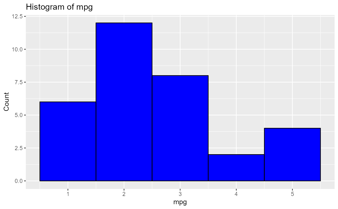
 # continuous data
ds_freq_table(mtcarz, mpg)
#> Variable: mpg
#> |-----------------------------------------------------------------------|
#> | Bins | Frequency | Cum Frequency | Percent | Cum Percent |
#> |-----------------------------------------------------------------------|
#> | 10.4 - 15.1 | 6 | 6 | 18.75 | 18.75 |
#> |-----------------------------------------------------------------------|
#> | 15.1 - 19.8 | 12 | 18 | 37.5 | 56.25 |
#> |-----------------------------------------------------------------------|
#> | 19.8 - 24.5 | 8 | 26 | 25 | 81.25 |
#> |-----------------------------------------------------------------------|
#> | 24.5 - 29.2 | 2 | 28 | 6.25 | 87.5 |
#> |-----------------------------------------------------------------------|
#> | 29.2 - 33.9 | 4 | 32 | 12.5 | 100 |
#> |-----------------------------------------------------------------------|
#> | Total | 32 | - | 100.00 | - |
#> |-----------------------------------------------------------------------|
# barplot
k <- ds_freq_table(mtcarz, mpg)
plot(k)
# continuous data
ds_freq_table(mtcarz, mpg)
#> Variable: mpg
#> |-----------------------------------------------------------------------|
#> | Bins | Frequency | Cum Frequency | Percent | Cum Percent |
#> |-----------------------------------------------------------------------|
#> | 10.4 - 15.1 | 6 | 6 | 18.75 | 18.75 |
#> |-----------------------------------------------------------------------|
#> | 15.1 - 19.8 | 12 | 18 | 37.5 | 56.25 |
#> |-----------------------------------------------------------------------|
#> | 19.8 - 24.5 | 8 | 26 | 25 | 81.25 |
#> |-----------------------------------------------------------------------|
#> | 24.5 - 29.2 | 2 | 28 | 6.25 | 87.5 |
#> |-----------------------------------------------------------------------|
#> | 29.2 - 33.9 | 4 | 32 | 12.5 | 100 |
#> |-----------------------------------------------------------------------|
#> | Total | 32 | - | 100.00 | - |
#> |-----------------------------------------------------------------------|
# barplot
k <- ds_freq_table(mtcarz, mpg)
plot(k)